Binary Search Tree(BST)

Different types of search tree includes Binary search tree, B tree, B+ tree,Red-black tree.
Basic operation takes time proportional to height of the tree in case of balanced tree.
  for complete binary tree with n nodes has worst case of Th(log n)
  for  linear chain of n nodes it behaves like linked list and has worst case of Th(n)
Can be used as dictionary and priority queue

Properties of Binary Search Tree

All nodes in the left subtree of parent must be no greater than parent that is key[left] <= key[parent]
All nodes in right subtree of parent must be no smaller than parent that is key[right] >= key[parent]

This property of binary search tree allows us to find sorted ordering in simple way by using inorder traversal

Tree Traversals

Process of visiting each node once.
Traversals are classified by the order in which root node is visited

1) Depth first traversal explores as far as along each node before backtracking
preorder (root left right)
inorder(left  root right) gives ascending sorted order
postorder (left right root)

2)Breadth first traversal
examining nodes at each level before moving to next level

Binary tree traversal implementation with Recursive procedure and auxiliary data structure require stack space proportional to the height of the tree. In a poorly balanced tree, this can be quite considerable.
Stack requirement can be removed by threading the tree, which will improve the inorder traversal alone.

Preorder traversal------------Th(n)

PREORDER-TRAVERSE(tree)
if (tree not empty)
  visit root of tree
  PREORDER-TRAVERSE(left subtree)
  PREORDER-TRAVERSE(right subtree)



Time complexity of recursive traversal 
consider n-node tree

T(n) = T(left)+ T(right) + d
T(n)=T(k)+T(n-k+1)+d
T(n) = Th(n)

Example Consider tree

       j         <-- level 0
     /   \
    f      k     <-- level 1
  /   \      \
 a     h      z  <-- level 2
  \
   d

inorder traversal   a d f h j k z
preorder traversal  j f a d h k z
postorder traversal d a h f z k j
breadth traversal   j f k a h z d

Reconstruction Property of Binary Search Tree
A unique binary search tree is possible from its its inorder, preorder and inorder, postorder but not from preorder and postorder. All the three a possible in case of full binary tree.


Example For 4 nodes draw a tree that gives same preorder and inorder traversal
It will have no left childrens

a
 \
  b
   \
    c
     \
      d
is the same possible with postorder and inorder traversal ?

Traversal with explicit Stack  
Every recursive call is Push operation and visit is print operation
The state of stack before first pop for
1) inorder
|_a _|
|_f__|
|_j__|
as in recursive call we call inorder(j) then on its left  inorder(f) and then inorder(a) then print(a) ...
2)  post order
|_a _|
|_f__|
|_j__|

3)preorder
|_   _|
|_ __|
|_j__|
before first pop


|_   _|
|_k _|
|_f__|
after first pop

Tree - Successor (x)       ----- O(log n)

successor in sorted order determined by inorder traversal
we need to find successor of node x

case1 : If the right subtree of  x is not null then need to traverse down and find
  Tree-Minimum(right(x))

case2 : right subtree of x is null then successor of x is
lowest ancestor of x whose left child is also an ancestor of x i.e

y = parent(x)

while(y!=null and x=right(y))

 x = y

 y = parent(y)

return y

Example Consider tree below and we want to find successor of node 13

                     15
                   /     
                 6
                   \
                    7  <-------y
                      \
                      13  <-------x
since right(y) == x so we move into loop

After first loop
                  15
                   /     
                 6 <-------y
                   \
                    7  <-------x

                      \
                      13
here also right(y) == x

After second loop

                  15 <-------y
                   /     
                 6 <-------x
                   \
                    7

                      \
                      13


right(y) which is null != x so we get 15 as ancestor of x


Time Complexity of Tree-Successor(x)
big O(h)


Inorder Traversal without using stacks 
If each node stores reference to parent then traversal implementation is possible without stack

or visited flag. When we don't have parent pointer we need to use Threaded binary tree.

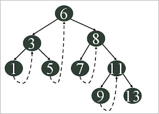
Right threaded binary 

We need to know if a pointer is an actual link or a thread, so we keep a boolean for each pointer.
Traversal
1) We start at the leftmost node in the tree, print it, and follow its right pointer
2) case 1  If its thread to the right, we output the node and continue to its right
    case 2  If we follow a link to the right, we go to the leftmost node, print it, and continue
Example
consider below right threaded tree

1)we start at leftmost node i.e 1, print it and follow right pointer
2)right pointer is  thread so we output 3 and move to its right
3)right pointer is link now to node 5 so we follow the leftmost node of 5 which is none so we print 5 and follow its right pointer and so..

Algorithm 

x  = leftmost(n);
while (x != null)
  print x
  If (right(x) = thread)
    x = x.right;
  else
     x = leftmost(x.right);

Advantages
Binary trees have a lot of wasted space: the leaf nodes each have 2 null pointers.We can use these pointers to help us in inorder traversals

Insertion and Deletion

Deletion----  O(logn)

Tree-Delete( T,z)
z is pointer to node of Tree T to be deleted
There are 3 possibilities

• deleting leaf node we modify the parent of z to replace z will null
• deleting a node with single child, splice z by making anew link between its child and its parent
• deleting a node with two children we splice out z, do not delete z instead choose either its inorder successor or predecessor and replace z with this and then delete successor 
• or for two children we can say delete smallest key in the right subtree or largest one in the left subtree

the successor of z,y will have no left child because if it has left child then it contradict that its successor of z.

Running time of deletion
running time of deletion procedure depends on Tree-successor which takes O(h) time
So running time of deletion is O(log n)


Insertion ------------ O(log n)
Tree-Insert(T,z)
point y to parent of each node
x to current node
while x!=null    // traverses tree downwards  takes O(h)
if key[z] < key[x]
 x=left[x]
else x=right[x]

at end y will hold the node where to insert z
p[z] = y

If y=null //means tree is null then create root
root[T]= z
else
set z as appropiate left or right child of y


Running Time
takes O(h) time

Build BST---------worst O(n^2)
In the worst case it takes O(n^2) when we have sorted list so all goes one after other in tree
making height of tree n
if we use self balanced tree it can be performed in O(nlogn)

Sorting ------worst O(n^2)
Build BST
perform Inorder traversal
worst case that of build procedure O(n^2)
poor cache performance and overhead of space
most efficient for incremental sorting



Range(a,b)
returns range of values a<=n<=b
find a and b in the tree
Let Pa and Pb be the search path from root to a and b resp.
Let x be the node where pa and pb split
for every node  v in the path a tox
if v > a
 print v
 inorder(right.v)

for every node  v in the path b to x
if v < b
 print v

 inorder(left.v)



Total time
finding the paths Pa and Pb takes at most O(h)
each inorder takes O(n) for n node tree
here we have k elements so O(k)
O(h+k)


Check the sequence if possible on searching
build the bst by placing larger on right and smaller on left
now check for each node every node in right subtree should be greater and in left should be small
Example
935, 278, 347, 621, 299, 392, 358, 363
isn't a possible sequence because 299 can't be in the right sub-tree of 347.

Problem Two binary search tree T1 and T2 with distinct nodes, each node in T1 is small than node in T2
Time complexity to merge T1 and T2 and height of new BST
Solution
If height of T1, h1, is greater than h2 then
find the largest element v of T1 and make it root
v= Find-Max(T1) //O(h1)
v.right =T2
v.left=T1
since maximum of T1 is less than T2 and will be greater than remaining T1
similarly when h2>h1 we can
Find-Min(T2) and make it root in time O(h2)

In both cases running time is O(min(h1,h2)) height of tree would be O(max(h1,h2)+1)

Tree Rotation
changes the structure without interfering with the order of the elements.
node node moves up(smaller subtree) other down(larger subtree)
Right rotation
                        a                right rotation                                 b
                      /    \              --------------                            /     \
                    b      c                                                           d        a
                  /   \                                                                         /    \
                d     e                                                                      e      c

AVL Tree
self balancing binary search tree
height of two child subnodes of any node differ by at most 1 or balance factor 1 0 -1
balance factor = height of left sunode - height of right
After each basic operation we perform rotations to keep tree balanced


Height of AVL tree
g(h)  number of nodes in the worst case the minimum number of nodes a AVL tree can have
g(h) = 1+ g(h-1)+g(h-2)
where g(0) = 1 and g(1)=2
interms of fibonacci sequence its
g(n) = f(n+2) -1
height of AVL tree is < 1.44 * log (n+2) - 1
Height of Red black tree is at most 2log(n+1)

Problem what is minimum number of nodes in AVL tree of height 10
Solution we know g(0) =1 and g(1) =2 and g(h) = g(h-1)+g(h-2) +1
so g(2) = 1+2+1 =4, g(3) = 7,g(4) = 12,g(5)=20,g(6)=33,g(7)=54,g(8)=88,g(9)=143,g(10)=232

Look up
look up is similar to unbalanced BST
since here its balanced in the worst also it takes O(log n)

Insertion
need to check ancestors for balance, if it becomes +- 2 we need to balance it
i)right-right case : when balance factor p for node is -2 that is right child outweighs
 check balance factor of right subchild (R )
   if p(R) <= 0 then left rotation with P as root
   if p(R)= +1 then double rotation wrt to P is needed first with R as root and next with P as root
ii) left-left case when balance factor for node P is +2 that is left outweighs

Dynamic Programming - LCS, Matrix Chain, Optimal BST, Knapsack

Dynamic Programming

• DP is general approach to solving problems much like Divide and Conquer, except that subproblems will typically overlap.
• Break the problem into reasonable number of subproblems in such a way that we can give optimal solution to subproblem to achieve optimal solution to large ones.
• The dynamic programming idea doesn't tells us how to find solution, it just gives us a way of making the solution more efficient once we have.

Top down solution and Bottom up solution
Bottom up solution involves recursive solution this is also usually done in tabular form
calculates smaller values first and then
build larger values from them
moves from f(0) to f(1) f(2) so on
Top down memoization store the result of caculation which are later used
first break the problem then
calculate and store its result
move from f(n) to f(n-1) f(n-2) ...

Difference from Divide and Conquer
Subproblem size is of additive order in dynamic programming that is little smaller than original problem but in  case of divide and conquer subproblem size is of multiplicative order that is its n times small than original problem


Types of DP problems

Dijkstra shortest path problem, Bellman Ford shortest path problem, Fibonacci sequence, balance 0-1 matrix,Tower of Hanoi,Flyod all pair shortest path

Longest Common Subsequence Problem

Given two strings: string S of length n, and string T of length m. Our goal is to produce their longest common subsequence, the longest sequence of characters that appear left-to-right (but not necessarily in a contiguous block) in both strings.

S = ABAZDC

T = BACBAD

LCS of length four ABAD

It is like finding  a 1-1 matching between some of the letters in S and some of the letters in T such that none of the edges in the matching cross each other.

Problem definition
consider two sequences
X =(x1,x2,...xm)
Y=(y1,y2,... yn)
Find longest common subsequence  Z=(z1,z2...zk)  of X and Y


Optimal substructure
1. If xm = yn that is last element is same then LCS also should have that last element

• zk = xm = yn because if it is not in Z then there exist some other sequence with xm that is longest
• remaining LCS will be of Xm-1 and Yn-1 
• LCS(X,Y) =(LCS(Xm-1,Yn-1),xm)

2. If xm != yn then either Z is common sequence which ends in 

•   yn i.e LCS(X,Y) = LCS(Xm-1,Y) or
•   xm i.e LCS(X,Y) = LCS(X,Yn-1)

Overlapping Substructure 
Finding solution now includes solving case 1 when x=yn or solving two possibilities for case 2
Solving both the possibility of case 2 needs to solve case 1 as their subproblems.

Recurrence Solution
c[i,j] be length of LCS of Xi and Xj which is
1) 0 when i=0 j=0
2)  c[i-1,j-1]+1  when i,j>0 and xi=yj
3)  max(c[i,j-1], c[i-1,j])  when i,j>0 and xi != yj

Using simple recursive solution will give exponential time, since there are Th(mn) distinct problems we use Dynamic programming to find solution bottom up.


Time Complexity
takes time O(mn)
space O(mn) if we want to retrace the path also
but if we need only the length we need to keep only two rows current and previous
The problem can be solved in polynomial time if number of sequences are constant but otherwise ........

Problem 

For X= 010110110 Y=10010101 Find LCS with matrix table

tracking back the LCS we get 010101

Matrix Chain Multiplication

Problem definition
Given A1, A2, …,An  compute the product: A1xA2x…xAn , find the fastest way (i.e., minimum number of multiplications) to compute it.

two matrices A(p,q) and B(q,r), compute their product C(p,r) in pqr multiplications

Different parenthesization will have different number of multiplications for product of multiple matrices.

There are an exponential number of different possible parenthesizations, in fact 2(n−1)C(n-1) /n or
P(n)   = 1 if n=1
         = sum(k=1 to n-1)P(k)P(n-k) if n>=2
catalan number, so we don’t want to search through all of them. Dynamic Programming gives us a better way.

Example: A(10,100), B(100,5), C(5,50)
– If ((AB) C), 10 *100*  5 +10 *5 * 50 =7500
– If (A(BC)), 10 *100* 50+100*5*50=75000
 The first way is ten times faster than the second

Denote matrices with their row columns as
A1(p0,p1), A2(p1,p2), …, Ai(pi-1,pi),… An(pn-1,pn)

so multiplying Ai..Ak Ak+1...Aj takes  pi-1 pk pj multiplications
that is multiplying A[2,2] and A[3,5] takes p1*p3*p5

Optimal Substructure
optimal parenthization of Ai,Ai+1...Aj splits the product between Ak and Ak+1  The parenthization of prefix subchain Ai...Ak must be optimal within Ai...Aj

Recursive Solution
Let m[i,j] be the minimum number of multiplications for Ai x Ai+1,…,x Aj where 1<=i<=j<=n
and thus for complete problem it would be m[1,n]
m[i,j]    = 0  if i = j
            = min(over i <= k< j) {m[i,k] + m[k+1,j] +pi-1pkpj } if i

Optimal Cost  and Overlapping Structure
Recursive solution will encounter the same subproblems  many time and hence running time becomes exponential but actual number of subproblems are Th(n^2), since one subproblem for each choice of i and j
that is C(n 2) + n
Tabling the answers for subproblems, each subproblem is only solved once. exploring the Overlapping structure

Running Time
O(n^3)
space Th(n^2)

Observations
we can fill the nodes A[i,j] where i=j and where j = i+1 initially
For solving each m[i j] we only use all the splits between i and j for calculation along with the cost to calculate
For A1A2A3A4 the nodes splits are like

Fig showing the split for A1A2A3A4

1-4 gets split into: 1-1,2-4;  1-2, 3-4;  1-3,4-4. similar for 1-2, 3-4; 1-3,4-4.
From the diagram we can find the order in which nodes are evaluated that is m[i,j]

Optimal Binary search Trees 

we are given n distinct keys and propabbility pi for each key that a search will be for ki
we also have dummy keys for key not in tree
Number of leaf nodes for  n keys = n+1

Probability of finding some search key key(success)  + probability of finding some dummy(unsuccessful) = 1

Assume that actual  cost of search is number of nodes examined i.e the depth of node found by search in T plus 1

Expected cost of search Tree  T is
E[search cost in T] = sum{0 to n} ((depth(ki + 1) * (pi) ) +sum{i=0 to n}((depth(di) + 1) * (qi))
1+ sum{0 to n} ((depth(ki ) * (pi) ) +sum{i=0 to n}((depth(di) ) * (qi))
because {sum 1 to n} pi + {sum 0 to n}qj = 1

expected cost of subtree when it becomes subtree of node
the depth of each node in subtree increases by 1
expected search cost increases by sum of all probabilities in tree that is  increase of
w(i,j)= {sum l= i to j} pi + {sum l= i-1 to j}qj  for nodes i to j in subtree 

Recurrence Relation
e[i,j] expected cost of searching an OBST containing keys ki ... kj.

e[i,j] =  qi-1 when j=i-1
        =  min{ e[i,r-1] + e[r+1,j] + w(i,j) }  when i≦j,i≦r≦j

Observations 
consider nodes  a, b, c, d in increasing order
with probability P(a) = .1, P(b) = .2, P(c) = .3, P(d) = .4


1) Possible BST

Fig. possible BST

search cost of node = (depth of node + 1) * probability of node
Average Cost = 1*0.4 + 2*0.3 + 3*0.2 + 4*0.1 = 2.0

2)OBST

   Average Cost = 1*.3+.2*2+.4*2+.1*3 = 1.8

Example 2

i   |   1     2    3     4    5
P  | .24 .22  .23  .3   .01

we find values of table e[i,j]
for i= j its
www.cs.wpi.edu/~songwang/ta/recitation6.ppt

 Knapsack Problem

Problem definition
we are given a set of n items, where each item i is specified by a size si and a value vi . We are also given a size bound S (the size of our knapsack). The goal is to find the subset of items of maximum total value such that sum of their sizes is at most S (they all fit into the knapsack).

Input:
Capacity of knapsack k
n items with weight wi and value vi
Output:
set S of items such that
sum of weight of items in S <= k
and sum of values of items in S is maximized

c[i,w] be solution for items 1,2..i for maximum weight w
When we are considering ith item either we include it or exclude it
If we include the ith item then value of that item will be added and remaining problem should give optimal soution for remaining weight that is c[i-1,w-wi ]
If we exclude the ith item then value then still we have weight w to fill and remaining i-1 items to check
that is c[i-1,w]

Recurrence Relation
c[i,w]         =     0     if i = 0 or w = 0
                  =    c[i-1, w]     if wi  ≥  w
                  =  max [vi + c[i-1, w-wi], c[i-1, w]}     if i>0 and w ≥  wi

Computing the maximum value in weight
 c[i, j] is table, that is, a two dimensional array,  c[0 . . n, 0 . . w]

for w = 0 to W
 c[0,w] = 0
for i = 1 to n

 c[i,0] = 0

for i = 1 to n
  for w = 0 to W
   if wi <= w // item i can be part of the solution
     if bi + c[i-1,w-wi] > c[i-1,w]

       c[i,w] = bi + c[i-1,w- wi]
    else

     c[i,w] = c[i-1,w]
   else c[i,w] = c[i-1,w] // wi > w

Example
consider  n =4 W=5 and following
weight and values (2,3), (3,4), (4,5), (5,6)

consider evaluation
for 1st row v1= 3, w1=2,

for c[1,1] w=1
since w1 > w 
   c[1,1]= c[0,1] = 0
for c[1,2] w=2
 c[1,2] = max(3+c[0,0] ,c[0,2]) = 3

 for c[2,1]  v2=4 w2=3 w=1

since w2>w, we have c[2,1] = [1,1] =0

for c[3,5] v3=5 w3=4 w=5

c[3,5] = max(5+c[2,1] , c[2,5])

similarly filling all we have

//incomplete
//travelling salesman problem
//all pair shortest path

Database Index - B tree, B+ tree

Why database index are used

Database index helps improve the data retrieval speed in response to certain search conditions.

Drawbacks with database index

slower write, index needs to be updated on sql updates

storage space, index may grow based on the column values

Type of Single level Database index

Fig. Sequential indexes

Ordering key field is used to physically order records on disk

Clustered index dictates the order of physical data in a table.

• can define only single cluster index on the table though it may have multiple attributes.
• clustering index has one entry for each distinct value hence non dense index
• when data is read in some sequential order or for some range it is efficient because it requires less data block reads.
• Some database define primary key as clustered index.
• If clustered index is defined on the primary key it is called Primary index.
• index entry is stored for only first record (anchor record)in each block, so its sparse index.
• Problem with it is insertion and deletion of records. Here we have to move the physical records as well as change the index entries also

Non Clustered index Data is present in random order in the table but ordering is specified by database index.

On the ordered index we can perform the binary search.

good for table whose values modify frequently.

Secondary index are dense and so one entry for each record and hence a secondary index needs more storage. There can be number of secondary index on table

 

Search Tree

Index sequential file has disadvantage that performance degrades as file grows.

the goal is to reduce the height of tree leading to less disk access

• search tree of order p has at most p children or
• (p-1) key values,ordered set of values, and p pointers, pointing to child nodes
• p1 k1 p2 k2 ....pq-1 kq-1 pq
• if any node has k children it has k-1 key values

Fig. search tree of order 4

Following condition for ordering of the keys

• each left node has key values less than parent node key value and each  right node key value greater than parent node key value
• keys in node are in ascending order

• Used for searching records on disk
• Each key value in tree is associated with a block or record pointer.
• the search tree itself can be stored on disk with each node stored in blocks
• insertion algorithms do not guarantee search tree is balanced which is important otherwise nodes at very high level would require many block access.
• deletion may leave nodes empty and may lead to more levels.

B Tree

B Tree has additional constraints that ensures balanced tree and not much space wastage on deletions

insertion and deletion are handled especially when node is full or when node becomes less than half empty on deletion

B Tree of order p is a search tree with order p with additional constraint that

• all leaves are on bottom level
• all internal nodes(except root) have at least ceil(p/2) nodes or it says each node should have at least half the maximum number of children
• root node can have as few as 2 children
• each leaf node must contain at least ceil(p/2) -1 keys

Fig. B tree of order 5

Here all internal nodes has at least ceil(5/2)= 3 children or 2 key values and each leaf node has at least 2 keys.

Any index structure other than B tree is subjected to overflow. Overflow is where any changes made to tables will not have records added into the original index structure, but rather tacked on the end.


Problem 1 Consider search field V= 9bytes block size B= 512bytes record pointer Pr=7bytes and block pointer Pb is 6bytes
How many childrens can a node have or order of tree so that each node can come in single block
Solution
let p be child pointer
a node consists of
key value + data pointer + child pointer
total size of key values ( p-1 ) * V
total size for data pointers (p-1)*Pr
total size for child pointers p*Pb
i.e (p*Pb) + (p-1)(V+Pr) <= B to fit in single block
p= 23


B+ Tree
variant of B tree datastructure
A B⁺ tree of order m is a tree where each internal node contains up to m branches (children nodes) and thus store up to m-1 search key values
order of tree measures the capacity of node or number of children nodes in internal node
B+ tree combines features of index sequential file organization with B tree
most widely used multilvel index implementation
For internal node
, where q <= p
For leaf node


where Pnext points to next leaf node
Requirements for maintaining B+ -tree
every node must contain at least ceil(n/2) pointers except for the root (which should have at least 2)
balanced: for ensuring good performance

Searching for key field value K

1) visit the root node, looking for the smallest key value greater than K. Suppose the value is Ki .
2) follow pointer Pi to another node
  - if K < K1 , then follow P1
    if K > Kmax , then follow Pmax
3) repeat step 2 until reaching a leaf node
Differences of B+-tree from B-tree

1. In B+ tree, data pointers are stored only at the leaf nodes

- more entires can be packed into internal (non-leaf) nodes of a B+ -tree than for a similar B tree meaning
B+ tree has larger fan out
- for the same block (node) size, the order p will be larger for the B+ -tree than for the B tree meaning   improved search time
- B tree eliminates redundant storage of search key values
- faster search in some cases to find desired search key values before reading a leaf node in B tree

2. Leaf and non-leaf nodes are of the same size in B+ tree, while in B tree, non-leaf nodes are larger
- complication in storage management for index structures

3. Deletion in B tree is more complicated
- in B+ tree, deleted entry always appears in a leaf
- in B tree, it can be a non-leaf node, requiring replacement by the proper value from the subtree of the node containing the deleted entry.

Problem 2 If maximum number of keys in b+ tree is 5 what is minimum number of keys in internal node and in root node.
Solution
Maximum number of childrens that a node can have(order of tree) = maximum number of keys + 1
so order of tree(b) = 5 + 1 =6
number of childrens in internal nodes(m)  is constrained by
ceil(b/2) <= m < =b
minimum number of internal nodes =  ceil(b/2) = ceil(6/2) = 3
so number of keys in that node = 3-1 = 2
 number of childrens of root node in b+tree is constrained by
2 <= m <=b
number of childrens in leaf node = no childrens of leaf node
number of keys in leaf node is constrained by
ceil(b-1/2) <= number of keys in leaf < = b-1

Problem 3
Consider a relation with 2M tuples stored in heap structure If we create a B+ tree index on this relation  with block filled to maximum capacity what would be size of tree . Assume following data
Disk page size B= 1000byte
key value(order key of relation) size V= 40bytes
disk page pointer Pb=10byte

Solution

If we were to calculate the maximum that can be stored we approach it top to bottom but if we have the entries that has to stored we approach bottom to top

Data record pointer will be stored in leaf pages since there are 2M tuples and its on order key so we will need 2M data record pointers but how many entries can a leaf page have

1) Find Number of entries a leaf page can have
leaf node stores same number of key values and record or data pointer along with a single next block pointer
so if we assume number of leaf entries to be n
n(V+ Pb) + Pb <= (size of page)  --since maximum number of entries should be allowed in a page
n = floor(size of page/(V+Pb))  -- ignoring the next block pointer for simplicity
n= 20

2) Number of leaf pages required to store 2M records = (Number of required index entries )/ (Number of index entries per leaf page)
= 2M/20 = 100000
3) Now we need to find number of entries that can come in internal nodes or branching factor m
consider number of index entries in internal node as n
each internal node will have a n-1 key values and n child pointers
(n-1)* V + n * Pb <= (B)
n =floor((B +V)/(Pb+V))
n=20

4) No we calculate Number of pages at level above leaf
there are 100000 leaf pages so we need this much index entries at level above it
so number of pages required at level above leaf = 100000 / 20 = 5000
Similarly we need to get to root that is when page is = 1
ceil(10000/20) ,ceil( 5000/20) ,ceil( 250 / 20), ceil(13 / 20) respectively for level above leaf
which is log20(100000) = 4
so we have total 5 level of pages and access to record would take 5 b tree block access  + 1 data block access = 6 disk access


References:
http://cis.stvincent.edu/carlsond/swdesign/btree/btree.html
http://www.cecs.csulb.edu/~monge/classes/share/ http://www.cs.sjsu.edu/~lee/cs157b/B_Trees_And_B__Trees.ppt
http://www.cs.virginia.edu/~son/662.pdffiles/662.physical.pdf

Serializability, Isolation Recoverability - Concurrency Control in Database

Why we want to run transactions concurrently?

Concurrent or overlapping execution of transactions are efficient

How we ensure the correctness of the concurrent transactions?

Concurrency control(Serializability) and Recovery are two criteria that ensure the correctness of concurrent transactions

Why concurrency control is needed

Lost Update : update of some data by one transaction is lost by update from another transaction
Dirty Read or temporary update problem : one transaction updates the value of common data and aborts before it can revert the changes transaction 2 reads the value of updated variable.
incorrect summary problem: transaction reads the data while another transaction is still changing the data

Why recovery is needed

In any kind of problem like hardware malfunction, software error exceptions or violating the concurrency property, deadlock recovery of transaction is needed

Transaction  states

• begin transaction marks the beginning of transaction. 
• end_transaction specifies transaction execution is complete and system check whether changes can be permanently applied.
• rollback or abort for unsuccessful end of tranaction

Fig. transaction states

• At commit point all transaction operations have been logged and new entry is done in log 'commit T' stating that all transaction operation permanently logged
• before writing commit T the complete log should be written to disk from buffers
• Rollback :  when commit T statement  is not found in log, its rollbacked

How recoverability is implemented

System log is kept on disk which logs transaction like write old value new value read.
Protocol that do not provide cascading rollback do not need to keep read entry

Schedules
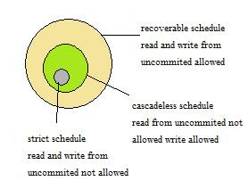
Recoverable Schedule : If T2 reads a data item written by T1 commit operation of T1 should appear before commit operation of  T2.

Cascadeless Schedule: If T2 reads a data item written by T1 commit operation of T1 should appear before read operation of T2.
Strict Schedule : If a write operation of T1 precedes a conflicting operation of T2 (either read or write), then the commit event of T1 also precedes that conflicting operation of T2.

Fig. schedules recoverability

pattern for recoverable schedule would be like

Fig. simple pattern for recoverability schedules on vertical time line

What is Serializability

If executing interleaved transaction results in same outcome as serial schedule(running transaction in some sequnence) then they are considered serializable. this schedule is type of nonserial schedule.

Serializabality might be compromised in some cases but recoverability compromise would mean violating database integrity. Isolation levels decide tradeoff between correctness and concurrency


Isolation level
when the changes made by one operation becomes visible to another operation
most relaxed ACID property
From more stringent to relaxed isolation levels
Serializable as if transactions execute in complete isolation, in serial fashion. read locks released immediately but write locks released at end of transaction
Read Uncommited Dirty reads allowed that is another transaction reads the data value but then first transaction can revert so other transaction has incorrect value
Repeatable read: A phantom read occurs when range of rows is read by one transaction and another transaction inserts or delete a record in between rows returned by same query is different at two points in time for a transaction that is another transaction updates and commits in between

Read commited(Non repeatable read):prevents dirty read that is reads commited data only.
UPDATE or DELETE of any of the rows read by earlier transaction

	Dirty Read	Lost Update		Phantom Records
Read uncommitted	yes	yes		yes
Read committed	No	yes		yes
Repeatable read	No	no		yes
Serializable	No	no		no

Types of serializability

View and conflict serializability

• conflict is subset of view serializability
• Conflict is widely utilized because it is easier to determine and covers a substantial portion of the view serializable

Equivalence to serial schedule such that

In view serializable, two schedules write and read the same data values.
and In conflict seriablizable, same set of respective chronologically ordered pairs of conflicting operations.


Conflict serializable
In conflict serializabability two schedules are conflict equivalent and we can reorder the non conflicting operation to get the serial schedule
Conflicting operation
1) they are upon same data item
2)At least one of them is write
3) they are from different transactions
Non commutative that is their orders matter

Testing conflict serializability
Test is through precedence graph. The acyclic preced graph shows conflict serialiczable schedule and topological sorting of that graph gives the serializable schedules
cycle of commited transaction can be prevented by aborting an undecided transaction on each cycle in precedence graph of all transaction

view serializability is NP complete
materialized conflict if the requested conflicting operation is actually executed
//pending

Problem 1 Consider two schedules
S1 : r1(x) w1(x) r1(y) c1
S2: r2(x) r2(y) c2
1.What the number of possible schedules.
2. How many serial schedules are possible
3. Determine type of schedules(recoverable cascadeless strict) and serializability(conflict seriablizable or not) for below schedules
S1: r 1 (X); w 1 (X); r 2 (X); w 2 (X); r 1 (Y); w 1 (Y); C 2 ; C 1
S2: r 1 (X); r 2 (X); w 1 (X); r 1 (Y); w 1 (Y); C 1 ; w 2 (X); C 2
S3: r 1 (X); w 1 (X); r 2 (X); w 2 (X); r 1 (Y); w 1 (Y); C 1 ; C 2 

Solution

1.
In general, given m transactions with number of operations n1, n2, ..., nm, the number
of possible schedules is: (n1 + n2 + ... + nm)! / (n1! * n2! * ... * nm!)
here m=2 and n1= 4 and n2 = 3
so (3+4)! / (3!*4!)
7C3 or 7C4
2.Number of serial schedules is m! where m is number of transactions
so here we have 2!

3. To check type of schedule
we need to check all conflicting operations of schedule 
S1 : r2(X) comes after w1(x) , since no commit before r2(X) its not cascadeless and strict
commit of T1 should be before T2 in this case for it to be recoverable which is not so it is not even recoverable. Its non recoverable schedule
S2: there is only one conflicting operation w1(X) w2(X) and for that we have commit of T1 before w2(X) so its strict schedule and so is cascadeless also
S3: for one of the conflicting operation w1(X) r2(X) there is no commit in between so its not cascadeless and strict. To check for recoverable commit of T1 should be before that of T2 which is there

To check serializability
S1 precedence graph is
T1 ---> T2
acyclic so its conflict serializable

S2 precedence graph
T1-------->T2
^                 |

|_________|

there is cycle so its not conflict serializable

//pending problems
http://academic.udayton.edu/SaverioPerugini/courses/Winter2006/cps432/index.html

Memory Management - Paging, Swaping, Partitioning

Bring process into main memory from input queue

Fix Partitioning

1. If using equal size partitions, main memory is divided into fix size partitions initially

• A process whose size <= partition can only be loaded in it. 
• If program large than partition size program has to design it with overlays reduces the OS overhead.
• Could lead to internal fragmentation for small size process
• Process can be loaded into any free partition.

2. If using unequal size partitions, main memory is divided into some unequal partitions initially.

• so a big process can be allocated the large size partitions and for a small size process we can allocate small partition reducing the internal fragmentation
• Process can be loaded in the smallest partition within which it fits.
• A scheduling queue is required for each different size partition which helps swapped out process.
• It minimizes the wasted memory from internal frag.
• But could lead to wastage when the large space remains unused because process will be queued for the other partitions that are smallest fit.

Fix partitioning leads to limit on multiprogramming that is active process in the system

Dynamic Partition

Dynamic partition leads to external fragmentation where portion of memory outside the variable size partition are fragmented.
Solution to external fragmentation problem is compaction to move the free space together.Its time consuming process and complete overhead. Processes must be dynamically relocatable for moving them around in memory
If we are to avoid compaction we can make intelligent assignment of process to memory so as to reduce the external fragmentation
Best fit First Fit and Next Fit. First fit is usually best and fastest.
First fit may lead to holes in the front end of memory. More the fragments in the front end more scanning for first fit



Next fit may lead to more external fragmentation leaving the need for compaction.
Best fits leads to many smaller memory holes leading to more frequent compaction.

Buddy System

compromise between two partitioning

Swapping

Consider at t0 we have some n process taking up the complete memory and at time t1 new process with priority higher than all the n process arrives.And we are using some priority scheduling then this process should get the CPU and should be brought in the main memory but since there is no space we need to swap out some process and bring high priority process in memory and then after its finished or some other swaps out we should swap that low priority process in .

Observations

Swapping was used in the old time sharing systems where memory was enough to load only single process so at end of each time quantum new process was brought in memory by swapping present process.
context switch time would be sum of swapping out and again swapping in process or part of it from backing store.
For efficient utilization of CPU each process execution time should be greater than the overhead i.e swap time.
Swapping is very expensive compared to instruction execution.
Swap time is dependent majorly on the transfer time, so if we move only that much portion of main memory which process is actually using, it would reduce the swap time.
We never swap the process with pending I/O or we execute I/O operations into operating system buffers only
Unix uses a variant of swapping, Demand Paging .

Paging

Allows physical address space of the process to be non contagious
Memory is divided into fixed small size chunks called frames and process into pages
Memory wasted in paging is only due to internal fragmentation and that only fraction in  last page of process.
Differs from fixed partitioning in that
 small partitions
 process can be allocated more that one partition
 non contagious allocation for process is possible
In simple partitioning logical address is location relative to beginning of the program and processor translates logical address to physical address
If Page size is decided as 2^n then remaining bits in the relative address of the process would decide the maximum number of pages allowed in page

In case of paging special hardware is used for logical address to physical address translation.Hardware looks up the logical address in the page table to find the physical address

Fig. logical address divided into offset and page number

Page table

stores mapping between logical address and physical address.
Contains one entry for each page of the process
operating system maintains a copy of page table for each process
Context switch time will increase as page table references need to be changed
If a page table entry is 4 byte long that is 32 bits it can address 2^32 physical page frames and if each frame is 4kb then we can address( 2^32)(2^12) = 2^44 bytes

Fig. lookup for virtual address in page table

Page Table Entry PTE

Each page table entry contain page frame address and property bits like a present bit, a dirty or modified bit, address space or process ID information.
Assuming 32-bit physical address with page size of 2^8, we  use 4 bytes for PTE (24 bit physical page number with 8 bits left for control.)

Sharing and Protection
Reentrant code, non self modifying code can be shared between different process
we map the re-entrant portion of code for each process into same physical frames.
the protection bits in the PTE helps perform certain validation like process is not trying to modify the read only page, that each reference to memory is valid.

Types of Page table

 Multilevel Page table

Since each process can occupy a huge amount of virtual memory that is it can have large number of pages that much entry for each process would be too high.To overcome this we store page table in virtual memory rather than real memory that is page table is divided into pages and when a process is running a part of its page table must be in memory including page that is executing

Fig. two level page table organization

All level page table are actually frames stored in the memory
Each entry in the page table is page frame address of size of  PTE


The format for multilevel page table specifies the offsets for each level page table


Consider  three level page table the logical address is divided into four part
1.offset into page directory or fist level page table.each entry points to page frame containing second level entries
2.offset into page middle directory or second level page table
3.offset into third level page table which specifies page frame
4.offset into page frame.

Fig. format of logical address for 3 level page table

Problem 1

Consider 32 bit Physical address 4KB pages, 4GB virtual address space
Number of pages in virtual address space 4GB/4KB = 2^20
Size of page table would be (PTE size) * (number of pages) = 4byte * 2^20 = 2^22 or 4MB
How many virtual pages would be required = (size of page table) / (size of page) = 4MB/4KB = 2^10
So, a top level page table would have 2^10 page table entries and total size would be = (2^10)(4bytes) = 2^12 i.e 4KB.Hence a two level page table would need 4KB more than single level page table. However, not all the second-level tables need to be resident in memory, and page tables are not needed for unmapped virtual memory. Thus the total usage is actually lower, and only the top-level table must be in memory at all times, requiring only 4KB (exactly one page) of physical memory per process.

Problem 2

consider a three level page table 36 bit physical address
2, 9, 9, 12 bits for first level second third and offset of page respectively
page frame size is 4KB and PTE is 4bytes
what will be number of bits required to address each next level table or page frame
Solution
First find Number of bits required to address a single page frame
Number of frames in the main memory =  (2^36/2^12) = 2^24
so we need 24 bits for addressing a page frame
Since each page table at each level is nothing but page frame addressed by PTE we need 24 bits to address each page frame
First level would be addressed by some process pointer after that each page table will have PTE to address next page frame.

Problem 3 consider a three level page table with
10,8,6,8 bits for first level second, third and offset of page respectively

1. What is the size of a page table for a process of 256K

Solution

Fig . three level page table organization for prob 3

Size of page table =(size of 3rd level table * number of third level page tables required + size of 2nd level        table *  number of second level page tables required + size of 3rd level table * number of first level page tables required)

Number of third level page table = (number of virtual pages) / (number of entries third level can hold)
To calculate number of third level page required we first find
how many pages are required by program or present in virtual address space
number of pages in virtual address space = (size of program ) / (page size)
                                                               = (256K)/2^8 = 2^10
so there should be 2^10 entries in the third level page table but each third level page table can hold 2^6 entries only so 2^10/2^6 =16 third level page table will be required

Number of second level page table = (number of third level page table)/(entries in each second level page    table)
                                                     =16/2^8 ~= 1

Number of first level page table = (number of second level page table)/(entries first level can hold)

                                                 = 1/1024 ~= 1
so size of page table = 1024*4*1+256*1+64*4*16

Note if different section are stored differently like data code stack, where two section could get same offset bits at second level then we need to store this in different page table. Number of second page table will change the first level will have three different entry for each section.

Problem 4 Consider system with 36 bit virtual address space and 8k page size with 4byte PTE.
If virtual address space of process is 8G analyze single two and three level page table organizations.
Solution
For first level page table number of page table
//pending

Inverted Page Table (IPT) with hashing
fixed size page table independent of number of processes and number of pages
entry for each physical frame in memory so if physical address is 32 bit with 8 bits for frame then there are 2^24 entries in the page table.
virtual address division = page number + offset but translation would be
page number portion is mapped into hash value which is pointer to inverted page table. since more than one virtual page number can give same hash value chaining technique is used
each page table entry holds page number,process identifier, control bits and chain pointer. Combination of pid and page identifies a page in virtual address space of a process. chain pointer may contains index value to address same table
system implementing IPT has difficulty implementing shared pages



http://www.cs.utexas.edu/users/dahlin/Classes/UGOS/hw/7bsol.html
http://www.ece.cmu.edu/~ece548/handouts/742sln1b.pdf

Process Synchronization in Operating System

Essential criteria to solve critical section problem

1.Mutual exclusion takes care of race condition.
2.Progress means that no process shall be kept from entering its critical section by another process that is stopped outside its critical section i.e if process j blocks in the remainder section it should not affect the entry of i in the critical section.
3.Bound waiting condition guarantees no starvation.If solution provides strict alternation then bounded waiting is inherently satisfied.If access to critical region is arbitrary then starvation is possible.



Mutual exclusion with Hardware 

1. Disabling the interrupts will ensure mutual exclusion but is not practiced for user processes and it is possible only in uniprocessor system. Disabling interrupt would ensure all 3 condition

2. Hardware provides special instruction that allows modification of a word or swap of words atomically
Test and set lock

• atomic(non interruptible) instruction used to write to a memory location 
• returns old value.
• no other process may begin test and set unless first is complete.
• guarantees mutual exclusion and progress but is prone to starvation. 
• starvation possible because access to critical region is in arbitrary fashion.  

initially set lock = false;

boolean TSL (boolean &lock) {
 boolean tmp = lock;
 lock = True;
 return tmp;
}

process p0 code
while(TSL(lock));
CS
lock = false;

gets the present value of the lock and sets it to true
Conditions
1.At time t0 process  p0 checks the while condition, TSL(lock) return false as lock is false initially, and sets lock = true, so p0 enters critical section.
2.At time t1>t0 process p1 tries to enter the critical section on call to TSL(lock)  it return true and sets lock to true again, so p1 is not allowed to enter critical section unless p0 executes the lock= false condition in exit section.
3.At time t2>t1process p0 has executed the lock = false and TSL(lock) returns false and p1 enters CS.

Exchange instruction (swap)
swap instruction executes atomically 
initially lock=false
code for process p0
key=true
while(key) swap(lock,key)
cs
lock=false;

Disadvantages of hardware instructions busy waiting(wasting cpu resource) and starvation possible.

Mutual Exclusion with software
1. Using lock variable alone does not ensures mutual exclusion.

Fig. software lock solution

2. Turn variable only.

3. Peterson's Algorithm

Allows two process p0 and p1 to share a single resource without conflict

Fig. peterson solution

1. Mutual Exclusion condition requires us to prove that if both process are checking the last statement of beginning section, that is while loop, only one of the process would be able to enter the critical section.
 Since value of turn can be either 0 or 1, turn value is not changed in CS or in remaining section, if it is 0 process 0 will enter and p1 would still be waiting and similar for p1.

2. For Progress we need to check if process blocks in the remainder section it does not affect the entry of other process in its critical section. In peterson solution process j set the flag[j] = 0 before entering in to its remainder section.so if process j now blocks in its remainder section then also process i can proceed with its critical section unlike in dekker's solution where if process blocks in the remainder section no other process can proceed to critical section.

3. Bounded waiting we need to check if one of the process is waiting that is in the while loop then eventually it will break out of loop and enter critical section.

Problems
All this solution has problem of
1. Busy waiting wasting cpu resource, frequent testing and waiting in while loop.
2. priority inversion problem
consider process p0 has low priority than process p1 and when p0 is in its critical section p1 comes, scheduler assigns CPU to p1 as its high priority process now
p1 gets CPU but cannot proceed because p0 is already in critical section(mutual exclusion)  while
p0 now waits for CPU assigned to process p1
process p1 gets into waiting state, before cpu could be assigned to p0 another process p2 arrives with priority less than p1 but greater than p0 this process will get the cpu
after p2 finishes p0 get the cpu and executes until it exits the critical section then p1 will get cpu
giving us priority inversion, low priority  process running before high priority process.

//here goes wake and sleep and it sproblems

4. Semaphores
Semaphore solution includes a semaphore variable and two atomic operations P(s) and V(s) semaphore is integer number representing the number of available resources.
if it is 0 means no resource is available and process has to wait.
if it is n means n resource are available and can be allocated.
V(s) executes when resource is released to increment the semaphore value.
semaphore does not distinguishes resources.
prevents race condition and deadlock does not guarantees them.

P(s):
while(1){

if s >= n

  s= s-n;

  break;
}

//here goes semaphore with waiting queue and wake up, sleep

semaphore with waiting queue can result in deadlock and also starvation if queue is LIFO


References

http://www.disi.unige.it/person/DelzannoG/SO1/AA0607/peterson.htm
http://en.wikipedia.org/wiki/Peterson%27s_algorithm
www.arl.wustl.edu/~fredk/Courses/cse422/sp03/.../concurrency1.ppt

Process Scheduling - Operating System Notes

Parameters affecting Process Scheduling decisions

• CPU utilization decreases by overhead of context switching.

• Thoughput is number of completed process per unit time and would increase if shortest task are executed firsts

• Turnaround time is time between submission of process and its completion. Average turnaround time is minimized by executing shortest tasks first

• Waiting Time time spent in ready queue. It is also minimized when shortest tasks are executed first

• Response time is increased if context switching is infrequent.
• response time is the (time of first result from system  - time of process submission)
• if process is submitted at time t0 and it is scheduled at time tn for for time t then response time is (tn+t) - t0

• run time of process = Turnaround time - waiting time 

• cpu utilization for n process = 

                    sum(run time of n process)/{sum(run time of n process) + sum(all contextswitch)}

• Penalty Rate = turnaround time / run time of process

• When calculating the turnaround time, waiting time response time, context switching time should be added it may be little when there are fewer context switch but may be significant as context switch increases.
• So by running shortest jobs  following parameters are optimized .
• Throughput , turnaround time, waiting time and also CPU utilization because no reorganization of the process queue is required, scheduling overhead is minimal.

Schedulers

• In Preemptive scheduling transitions from running to ready state .Special hardware is required for preemptive scheduling ,affects the design of kernel

• The scheduling algorithm in which there is  prioritization or are premptive may lead to starvation because a high priority process will always  hog the cpu.there wont be starvation in non premtive scheduling

First Come First Serve (FCFS) process scheduling

• cpu utilization is optimal because least possible context switch, on process completion only

• Throughput, turnaround time, average waiting time and response time not optimal as long process can hog the cpu.

Shortest  Job First (SJF) non premptive process scheduling

• CPU utilization is optimal

• Average waiting time is optimal among all non preemptive schedulings

• throughput is optimal in all non preemptive scheduling

Shortest Remaining Time First (SRTF) premptive SJF process scheduling

• includes overhead of more context switching and also to position the process in queue

• CPU utilization not optimal as context switch increases
• maximum throughput if correct estimates for cpu burst and if context switch negligible
• Average turnaround time is less than SJF as newly arrived short burst process would be executed first which reduces the waiting time of short burst process.
• Starvation is possible.

Round Robin (RR) scheduling

• High context switching hence low cpu utilization
• optimal response time
• thoughput between FCFS and SRT
• no starvation. 
• round robin is good for short jobs
• Average turnaround time is greater than in SJF  but average waiting time is less than in SJF
• If time quantum q is increased ,

•  Average Turnaround time will decrease

•  Average waiting time will increase

• FCFS is RRS with infinite time quantum

Observations about Round Robin scheduling
if we have process p1 with alternating burst of t1 for cpu and t2  for i/o the result of the computation will be visible only after the i/o is done that is response time would be t1+t2 and not t1
Response time if all n process are active then response time = n*(q+s) under certain conditions when q is greater than cpu burst
Two i/o operations of process p1 and p2 are performed in parallel if they wait for different resource, until specified otherwise , that is p2 does not have to wait



Problem 1  Consider n processes sharing the CPU in a round-robin scheduling.  Assuming that each process switch takes s seconds, what must be the quantum size q such that the overhead resulting from process switching is minimized but, at the same time, each process is guaranteed to get its turn at the CPU at least every t seconds (i.e., it is idle for no more than t seconds between time slices)?

Solution

next execution of the process should occur within t seconds

Each process runs for q period and if there are n process
p1 p2 p3 ..... pn p1 p2 ... then p1 turn comes again when it has completed time quanta for remaining process p2 to pn  i.e it would take at most (n-1)q time
So Each process in round robin gets its turn after <= (n-1)q time when we don't consider overheads
but if we consider over head(s) then it would be ns+(n-1)q
So we have ns + (n-1)q <= t
overhead will be reduced when time quantum is maximum allowable i.e,  q = (t-ns)/(n-1)

Problem 2 consider 10 identical process intiated at same time with 15 identical requests
Each request consumes 20 ms of CPU A request is followed by I/O that consumes 10ms The scheduling overhead is 2ms. Find response time for first and last request when
1) time quantum q >= 20ms and
2) time quantum q =10 ms
Solution
Gantt chart
p1 s p2 s p3 s .................p10 s p1 s p2 s ........p10 s p1 s
first requests                               second requests for each process
assuming output recieved after q+s
response time for first process first request = 20 + 2 = 22ms
response time for last process first request =  (20+2) *10 = 220ms
For second run each process first spends 10ms in the I/O wait then makes request
so time quantum q will be spent as
10msec i/o wait + 10 cpu
second request is made after 10ms i/o wait
and result of second request will occur on third run after completing the 10ms CPU
response time for first process second request = 10(on second run)+2+ 9(20+2) + 10(third run) = 10*(20+2)
similarly for all other processes also same time would be incurred

when q=10ms
that is even the first request will not complete on first run
(10+2)*10 // first completion
10+2  //now 20ms CPU for process 1 completes
that is 11*(12)ms for completion of first process first request
For last process it would be (10+2)*10+(10+2)*10 = 240ms
For subsequent request each has to spend one cycle in I/O and then similar way we have to add above time

//pending
link

Refrences
http://en.wikipedia.org/wiki/Scheduling_(computing)
http://read.cs.ucla.edu/111/notes/lec7?do=index
http://people.engr.ncsu.edu/efg/501/f97/solutions.html