Operating system Problems

Deadlock problems
Things to Remember
1)Using Banker Algorithm you always work on NEED not MAX claim
2)We add the Allocation NOT  the NEED to Avaiable
3)Available resources, when total resources is given = total - allocated
4)when a new process enters the system find its need request and new available as
new available = available = request for process
5)A process might not be in deadlock or safe state then it is in unsafe state that is a process might not request the maximum need and so wont go in deadlock
6)Deadlock can involve process not in circular chain if they request resource currently held by process in circular chain
7)When available is greater than need of every process we have safe sequence

Problems
Problem Consider p processes each needs a max of m resources and a total  r resources are available. What should be relation between p,m,r  to make the system deadlock free?

Solution:
The worst case is when every process is holding m-1 resource and a process requests 1 more resource and that cannot be fullfilled if we only had one more resource we can allocated any process that resource and full fill others need also  So total number of resources should be

r > (m-1)*p

we can prove that system can safely reach the state where each process is allocated m-1 resource


We can also interpret above equation as
mp < r + p
that is sum of all the resource need of all process should be less than r+p

Problem A system has 3 processes and 4 available resources with max need of each process as 2
Prove that system is always deadlock free
Solution we check the worst case we derived above that is
r>(m-1)p
here m=2 and p=3 so r should be greater than 3 Hence its deadlock free


Detect Deadlock from code
whenever we are asked to find if the system is in deadlock we have to look if
1)request of the form below and
2)processes p0 and p1 executed simultaneously

p0                       p1
Request Ri     request Rj
request Rj      request Ri

 Problem

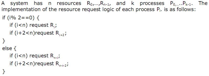
Solution:
Even processes requests
Ri
Ri+2
that is requests resource i and i+2 from beginning

odd process requests
R(n-i)
R(n-i-2)
that is ith and i-2 from last

consider even process as index i and odd as j
Now system can be in deadlock when

1)Ri = Rn-j-2 that is
i = n-j-2
i+j = n-2
and
2) i+2 = n-j that is
i+j = n-2

So we have equation  i+j=n-2
if this is satisfied for any two processes then only deadlock is possible
but we know that i is even and j is odd so
1) i+j is odd and RHS n-2 can be odd only when n is odd and also
2) if number of process are k then i and j has to be < k

Lets see for
1)n=41 and k=19
n-2 = 39 and maximum j can be 19 and i 18 which combine donot ma ke 39 so no deadlock possible
2)when n=21 and k=12
we have n-2 = 19 and i max can be 12 and j 11 which can make the total sum so lets check
when i =10 and j=9 . yes we have deadlock

Scheduling Problems
Things to Remember
In round robin overhead is minimized when time quanta q is maximized
In round robin we use queue order that is does not necessarily
Convoy effect when process needs to use resource for a small time but other process is holding it for long time. FCFS scheduling may suffer convoy effect.
I/O bound process do not use their entire CPU quanta. Better utilization by giving high priority to I/O bound process because of convoy effect


Problem

Use time q=5ms

Solution
Round robin
Shown below is gantt chart with queue

waiting time
total time that is time from arrival to completion - time executing (given in table)
for P1 : 55 - 20 = 35
for p2 : (77-4) - 32= 41
for p3 : 59-14-9 = 36
for p4 : 65-12-11=42
Average 38.5


Shortest Job first
p1 p4 p3 p2
Average = 17.75


Shortest Remaining First




Problem Consider Exponential average to predict length of next CPU burst
1) a=0
then system always uses past history to predict CPU burst without taking in account the recent observation
2)a=.99
then gives very high weight to recent observation and very less to past history and hence almost no memory is required for history


Problem 10 i/o bound process and 1 cpu bound process Each I/O bound process issues I/O operation once for every 1ms of CPU computing and each I/O takes 10ms to complete . context switch overhead = .1ms What is CPU utilization for
1)q=1 ms
Solution CPU utilization is (execution time )/(execution time + overhead time)
for each time quanta system incurs cost of .1 so
1/1.1 = .91
2)q=10ms
A cpu bound process will run for 10ms then a context switch of .1ms total 10.1
each i/o bound process interrupts cpu to context switch for I/O activity after 1ms so total is 1.1 and for 10 process would be 10*1.1
for a execution time of 20ms we have
CPU utilization  = 20/21.1 = .94

Multiprogramming
If a job spends p fraction of time in I/O waiting then
with sequential execution CPU utilization is 1-p
If p =.60 that is its spending 60% of time doing I/O then CPU utilization is only 40%
For multiprogramming with n jobs in the memory
probability that all n processes are waiting for I/O is p^n
CPU utilization is 1-P^n that is probability that at least one process is ready for CPU
this is on the assumption of no cpu overhead

Problem  Suppose two jobs, each of which needs 10 minutes of CPU time, start simultaneously. Assume 50% I/O wait time.
a) How long will it take for both to complete if they run sequentially?
solution Each process takes total of 10 min for I/O + 10 min for CPU that is 20
Total time for complete T = 20min +20min = 40mins
b) How long if they run in parallel?
probability p for which time is spent in I/O
p = 1/2 //50% I/O
CPU utilization = 1-p^2 = .75
T*.75=20


File system
Inode
A files block are scattered randomly
Inodes keeps pointer to data blocks
Each Inode has 15 pointers
First 12 points directly to data block
13th points to indirect block that is block containing data block
14th points to doubly indirect block that is points to block containing 128 addresses of indirectblock
15th points to triply indirect block that is block which points to doubly indirect block
Consider block size of 4K as in unix file system
then 12 direct block pointer can point to 12*4K =48K
if each pointer is of 4 byte then a single block can accomodate 4K/4 = 1K
one indirect can point to 1K*4K =4MB
one doubly indirect 1K*1K*4K

Problem  Let there be 8 direct block pointers, and a singly, doubly, and triply indirect pointer in each inode and  that the system block size and the disk sector size are both 4K. If the disk block pointer is 32 bits, with 8 bits for identifying physical disk, and 24 bits to identify the physical block, then:

1)maximum file size?
Solution each block can hold = 4K/4 = 1K pointers
so direct blocks = 8*4K
single indirect =1K*4K
double indirect =1K*1K*4K
triple indirect = 1K*1K*1K*4K
all sums around 4TB

2)what is maximum file system partition size
Since disk block pointer is 32 bit it can point 2^32 blocks
which includes 8 bits to identify physical disk and 24 bits to identify block
since each block is 4K so total = 16TB

3)assuming inode in memory how many disk access are required for byte position 2634012
since each block is of 4K we find the offset 2634012 modulo 4K = 284  and block number is 643
this block will be addressed by single indirect block so number of access = 1for accessing indirect block and 1 for accessing the actual block =2


Memory Management

.

Remember to always add the time to check cache or tlb even when we have miss.

Problem Assuming single level page table If a memory reference takes 100 nanoseconds, time for memory mapped reference is ?
i)when no TLB
 100 for accessing Page table and 100ns for accessing actual data frame
ii)TLB with access time 15ns and .9 memory hit in TLB
 if page number is present in TLB then 15+100
 if page number not found in TLB then 15+100+100
Hence EMAT = 115*.9 + 215*.1

Problem Consider demand paging with the page table held in registers, memory access times
8 msecs for  page fault if --  empty page is available or the replaced page is not modified,
20 msecs if the replaced page is modified
70% of the time the page to be replaced is modified
100 nsecs memory access time


What is the maximum acceptable page fault rate (P) for an effective access time of no more than 200 nsecs?
Solution
p = page fault rate
and m be percentage of time page is modified then

EMAT >= 1-p(memory access time) + p (m (time to write back dirty page & service fault) + (1-m)(time to service page fault))

.2 >= 1-p(.1)+ p (.70*20000 + .30*8000)

Problem Consider average size of a process as p, size of a page table entry is e, what page size minimizes wasted space due to internal fragmentation and page table?
 Solution
page tables used to store the frame number and control bits is actually a overhead or wasted space
so we calculate wasted space  = space used by page table + space wasted due to internal fragmentation
avg number of pages =p/s
and total size of all pages =pe/s
avg space wasted due to internal fragmentation s/2

so total waste = pe/s + s/2
to find min take derivative
- pe/s^2 + 1/2 = 0
 pe/s^2 = 1/2
 s = sqrt(2pe)

 
Problem Consider the average process size is 128 KB and the number of page entries is 8. What will be appropriate page size
Solution



Page replacement
one has reference time highest means it was referenced farthest on left 
FIFO doesnot depend on the reference time but on the load time
NRU replaces one with r=0,w=0
second chance replaces earliest page with r=0
 If you are given page has been modified written to or dirty then it takes 2 I/O for replacing that page
1 to bring in new page and 1 to write back this page
Virtual to physical address binding takes place during runtime

Consider the following piece of code which multiplies two matrices:

int a[1024][1024], b[1024][1024], c[1024][1024];
multiply()
{
   unsigned i, j, k;
   for(i = 0; i < 1024; i++)
       for(j = 0; j < 1024; j++)
           for(k = 0; k < 1024; k++)
               c[i][j] += a[i,k] * b[k,j];
}

Assume that the binary for executing this function fits in one page, and the stack also fits in one page. Assume further that an integer requires 4 bytes for storage. Compute the number of TLB misses if the page size is 4096 and the TLB has 8 entries with a replacement policy consisting of LRU.

Solution:

1024*(2+1024*1024) = 1073743872
The binary and the stack each fit in one page, thus each takes one entry in the TLB. While the function is running, it is accessing the binary page and the stack page all the time. So the two TLB entries for these two pages would reside in the TLB all the time and the data can only take the remaining 6 TLB entries.
We assume the two entries are already in TLB when the function begins to run. Then we need only consider those data pages.
Since an integer requires 4 bytes for storage and the page size is 4096 bytes, each array requires 1024 pages. Suppose each row of an array is stored in one page. Then these pages can be represented as a[0..1023], b[0..1023], c[0..1023]: Page a[0] contains the elements a[0][0..1023], page a[1] contains the elements a[1][0..1023], etc.
For a fixed value of i, say 0, the function loops over j and k, we have the following reference string:

a[0], b[0], c[0], a[0], b[1], c[0], ¡ a[0], b[1023], c[0]
¡
a[0], b[0], c[0], a[0], b[1], c[0], ¡ a[0], b[1023], c[0]

For the reference string (1024 rows in total), a[0], c[0] will contribute two TLB misses. Since a[0] and b[0] each will be accessed every four memory references, the two pages will not be replaced by the LRU algorithm. For each page in b[0..1023], it will incur one TLB miss every time it is accessed. So the number of TLB misses for the second inner loop is
2+1024*1024 = 1048578
So the total number of TLB misses is 1024*1048578 = 1073743872
Partitions
It is possible to get the new block from the external fragmentation

Problem Consider following hole sizes in memory in  this order: 10KB, 4KB, 20KB, 18KB, 7KB, 9KB, 12KB. Which hole is taken for successive segment
request of 12KB, 10KB, 9KB for
a. First fit?
20KB , 10KB,18KB
b. Best fit?
12KB, 10KB,9KB
c. Worst fit?
20KB,18KB,12KB
d. Next fit?
20KB,18KB,9KB

Secondary storage problems
Problem Consider
10000 RPM spindle speed,
300 Sectors per track,
512 Bytes per sector,
9801 cylinders (tracks per platter side),
24 tracks per cylinder (12 platters),

6ms average seek time,
0.6 ms track-to-track seek time.

Suppose you want to read a 4,608MB file under the following two sets of assumptions:
a) Assume the file is allocated consecutive sectors and tracks on one surface of one of the platters. How long does it take to read the file’s data and what is the average throughput?

Solution
total time to read file =avg seek time+ avg rotational delay + transfer time
rotational delay = 60s/m  / 10000rev/min= 6ms /rev

Calculate bandwidth
total number of bytes in track = total number of sectors * number of bytes per sector = 300*512 = 153600 bytes/sector
bandwidth = number of bytes in track/ rotational delay = 153600/6 bytes/sec
transfer time for x bytes = x/bandwidth = 6*x/156300

For file
Number of blocks in file = 4608000 / 512 blocks = 9000 blocks
or total of  30 tracks

transfer for first track T1 = average seek + average rotational + transfer time
=6ms+3ms+6ms =15
For remaining tracks it would be 6ms transfer time for track + .6ms track to track time
6.6*29
total time =15 +6.6*9
average throughput is 4608000/total time



b) If the individual blocks are randomly scattered over the disk how long will it now
take to transfer this file and what is the average transfer rate?



we read each sector with same avg rotational delay and  avg seek time
so each request is uniform with time of 6ms avg seek time+3ms of avg rotational dealy+6/300 to read a sector =9.02
and there are 9000 such sectors so total time would be 9000*9.02ms

Graph Algorithms

Minimum Spanning Tree

Problem definition
In a weighted connected graph G(V,E,W) Find tree T that contains all the vertices in G and minimizes the sum of weight of all edges
Greedy approach to find minimum spanning tree,at each step one of the several possible choices is made that best choice

Safe edge is one that can be added to  subset of edges of minimum spanning tree A without violating the condition
A cut is any partition of V
If no edge in A crosses the cut then it respects the cut
An edge is light edge crossing the cut if its weight is minimum of any edge crossing the cut

Theorem In graph G if we partition set V into S and V-S and A is subset of edges of minimum spanning tree then a light edge {u,v} can be added to set A safely that is AU{u,v} is also subset of MST
If  edge u,v is not part of MST then there must be some other edge (xy) connecting the two partitions V  and V-S so if we add edge uv to it, it should create cycle but we have uv as light edge so
w(uv)<=w(xy)
so we have MST with uv also
But if all edges have distinct weights we cannot have this condition and only edge {u,v} can be part of MST

Generic- MST : Find a safe edge and add it to A to form MST

Kruskal algorithm
greedy algorithm because at each step adds the least possible weight edge to A.
set A in case of Kruskal algorithm is forest
It finds a safe edge to add to the growing forest by finding edge {u,v} of least weight that connects any two trees in forest

Kruskal algorithm
Kruskal(G,w)

For each vertex v in V(G)
  make-set(v)   //O(V)
sort the edges of G in nondecreasing order by weight   //greedy approach to take minimum weight
For each edge E{u,v} in the sorted list
if both endpoints do not belong to same tree then  //if belongs to same tree then we would have cycle
If Find-Set(u)  != Find-Set(v)          //O(E) for each edge
 then A =A U {u,v} // add edge E to set A
 Union(u,v)

we used disjoint set data structure to implement it

Running time
depends on the disjoint set operations
time to sort the edges takes (E log E)
creating a disjoint set of vertices that is that many number of distinct trees initially and the main loop to process each edge takes O(E+V)a(V), but since G is connected graph E >= V-1 and so it becomes O(E)a(V) (a takes into count the union at last when vertices are added to tree) where a(V) is (log V) = O(log E)
Total running time is O(E log E) also |e|<=|v|^2  so log E = O(log V) and we can also state running time as
O(E log V)


Prim Algorithm
also example greedy algorithm 
edges in the set A forms Tree that is it works by adding edges to a set A
operates like Dijkstra algorithm
It gradually creates a minimum tree that spans all the verties
At each step light edge is added to tree A that connects A to an isolated vertex
key concern is how to select
min priority queue is used to hold vertices not in tree A based on key field .For each vertex v, key[v] is the minimum weight of any edge connecting v to a vertex in the tree

Prim Algorithm
r is the starting vertex
At each step we update the adjacent veritces weight so that when we call extract-min on priority queue we get the light edge that is minimum weight edge
Prim(G,w,r)
for each vertex add set the key field to infinity and parent field to null except for the vertex r for which key field is set 0
set the min priority queue with this information
while queue is no empty
  u =  extract-min (Q)            // we process vertex in order on min key in Q
  for each edge v adjacent to u
   if v is in the priority queue and weight w(u,v) < key[v]  
    update the key and parent for vertex u

For every vertex v in Q, key[v] is the minimum weight of any edge connecting v to a vertex in the tree
Q will have non infinite key for those vertexes whose adjacent vertex has been processed or in other words we determine the cut of the graph and light edge is added to the set A.
set A and Q forms disjoint sets of cut.


Loop invariants
set A contains V-Q that is vertices processed and removed from queue
for all vertices in queue if parent is not null then key of vertie

Running time of prim algorithm
depends on how min priority queue is implemented
1)If binary min heap is used
we use build min heap to create vertex with key and parent fields it will takes O(V) time
 Extract min takes O(log V)  //when selecting the vertex in queue
and is called V times that is for each vertex  so extract min takes total of O(V logV)
Decrease key on binary heap = O(log V)  // when updating the key of adjacent vertices
and is called for all the adjacent vertices of v
sum of lenght of all adjacency list is 2|E| so decrease key is called O(E logV)
total time is O(V log V + E log V )
when graph is sparse we have e << v^2 and e = Th(v) so cost is O(V log V)
when graph is dense we have e ~= v^2, so cost is O(V^2 log V)
2)using fibonaci heap
extract min can be performed in O(log V)
and decrease key can be performed in O(1)
so total time is (VlogV+E)
for sparse we have e=Th(v) so  cost is O(VlogV)
for dense we have e ~= v^2 so cost is O(V^2)
3)using adjacency matrix
scans the list to find the smallest key   O(V)
 for each vertex update its adjacent vertex weight   //O(deg(u))
total cost is {sum over all vertices} O(V + deg[u])
so  total cost is O(V^2 + E) =O(V^2)

Negative edges in Kruskal and Prim algorithm
Negative edges does not affects the kruskal algorithm Both works correctly as should be
Light edge donot distinguish negative and positive edges

Shortest Path Problem

There is only one minimum spanning tree but in general there is different shortest path for each source

Optimal structure
each subpath of shortest path is shortest path

Cycle in graph
negative weight edges
there may be negative weight edges
If G contains no negative weight edges then shortest path weight remains well defined for all sources s
If there is negative weight cycle reachable from s then shortest path are not well defined
If there is negative weight cycle on some path from s to v then shortest path weight d(s,v) = -infinity

If vertex v is not reachable from s than d(s,v) = + infinity

Dijkstra algorithm requires no negative weight edge in the input
Bellman Ford algorithm allows negative  weight edge in input graph and produces correct answer as long as no negative weight cycles are reachable from source. It can detect the negative weight edge cycles and reprot there existence

Shortest path cannot contain negative edge cycles and also not positive weight edge cycles
zero weight edge cycle it can be on the shortest path but then we can also go via another path instead of zero cycle
So we will consider shortest path only for v-1 edges that is without any cycle

Relaxation step
Relax(u,v,w)  //relax edge {uv} having weight w
we update the distance on the vertex v like
if d(v) > d(u) +w(uv)
then update d(v) with d(u) + w(uv)

Each algorithm differs in how many times and in which order they relax edges.
Dijkstra algorithm relaxes each edge exactly once
In Bellman ford each edge is relaxed many times

Bellmand Ford Algorithm
solves single source shortest path in weighted directed graph G(V,E)
negative weight edges allowed
detects reachable negative weight edge cycles
algorithm returns boolean value indicating whether or not negative weight edge cycle exist If such cycle exists the algorithm indicates there is no solution If there is no cycle it  produces shortest path and weight

algorithm return TRUE if and only if the graph contains no negative weight cycle reachable from source s

Bellman-Ford(G,w,s)
Initialize(G,s )  //initializes the d(v) for each vertex to infinity and path s to zero
for i =1 to |V|-1  //remaining vertices other than source
  for each edge (u,v) in E(G)  //each pass relaxes each of the edge of the graph so |v-1|*|E| relaxation
    Relax(u,v,w)
for each edge (u,v) in E(G)   //check negative weight cycle
 check if d(v) > d(u) + w(u,v) 
    return FALSE              //if negative weight cycle exist
return TRUE

Running Time
Initialization takes O(V)
we relax each edge for each vertex that is O(VE)
check for negative cycle takes O(E)
total running time is O(VE)

For proving the correctness of the bellman ford we need to prove that each vertex v has shortest distance from s that is for each vertex v d[v]=shortest distance from s

Observations
does not always returns shortest path from s to t in all the graphs, when graph have negative weight cycle
If graph has all distinct vertices then shortest path between two vertices may not be unique, same weight path possible


Dijkstra algorithm
single source shortest path on directed weighted graph
no negative edges allowed
example of greedy algorithm
greedy algorithms doesnot always yields optimal result but in case of Dijkstra it return optimal weight path 
maintains set S of vertices whose final shortest path weight from source have already been determined
select vertex u whith minimum path estimate from remaining vertices and adds it to S and relaxes all edges leaving u

Dijkstra (G,w,s)
Initialize all vertices to infinity distance
build a min priority queue from vertex set V[G] //Q would always contain V-S
while priority queue is not empty    //runs for |V| times
 u = extract-min(Q)
 add u to S
 for each vertex v adjacent to u
  relax(u,v,w)

Running Time of Dijkstra
maintains min prioity queue by calling three operations
Insert(build heap) ,Extract-min(G) and Decrease-Key(Relax)
1)we take advantage of the vertices being numbered 1 to |V|-1
we can perform Insert and Decrease-key in O(1) and extract min in O(V) time
total running time O(V^2+E) = O(V^2)
2)If graph is sparse that is E =o(V^2/log V) we implement it using binary min heap
build heap O(V)
extract min O(log V) and there are V such extract so O(V log V)
Decrease key O(log V) , number of decrease key is of O(E) so total  O(ElogV)
Total running time = O((V+E)log V) = O(E log V)
3)with fibonacci heap we can achieve (V logV+E)

Observations
Dijkstra algorithm relaxes each edges only once
example when Dijkstra algorithm does not works
here we start from A relax edge AB and AC
B gets labeled (5,A) and C(10,A) So we choose B and relax edge BD, D gets new label (6,B)
D is processed then C is chosen and edge CB is relaxed and B gets new label (3,C)
D has label (6,B) while D should have been (4,B)

All pair Shortest Path

Breadth First Search
for searching graph
given graph G and source s BFS explores the edges of G to discover every vertex that is reachable from s
It computes the smallest number of edges from s
explores all vertices at distnace k from s before moving to k+1 vertices

To keep track of progress, colors each vertex white gray or black.
not processed white
when first encountered it becomes non white
three color for vertices
white -- not discovered yet
gray discovered but not processed
black all the adjacent vertices discovered and grayed


all vertices adjacent to black are discovered vertices
vertices adjacent to gray may not be discovered

constructs a breadth first tree initially containing only its root

FIFO queue used to process vertices in order in which they are discovered

BFS(G,s)
color each vertex white initially , their distance infinity
color sources s as gray that is processing starts with s
enqueue s
for each vertex in queue
u = dequeue(Q)
for each adjacent vertex v of u
if its not discovered yet that is color ==white
color it gray
increase weight by one d(v) = d(u)+1
enqueue(Q, u)
color v black that is all its adj have been discovered

Queue Q always consists of gray vertices


Running time
aggregate analysis
Enqueue and Dequeue O(1) time
each vertex is enqueued and dequeued once giving O(V)
since sum of lenght of all adjacency list is Th(E)
total time scanning adjacency list is O(E)

total running time of BFS is O(V+E)

breadth first search shortest path, that is, minimum number of edges or weight of 1 on each edge, for each vertex
if it is reachable else infinity

DFS
edges are explored out of most recently discovered vertex
when all edge o v has been discovered search backtracks to explore edges leaving the vertex from which v was discovered
predecessor graph of DFS may be composed of several trees unlike that or BFS

like BFS vertices are colored to indicate their state
white initially grayed when discovered and black when finished

DFS(G)
initialize each vertex color to white
time =0
for each vertex in V[G]
if we have white colored vertex call DFS-VISIT(u)

DFS-VISIT(u)
set color of u to gray indicating its discovered
time = time+1
d[u] =time // time when vertex u is discovered
for each vertex v adjacent to u
if it is white colored
then call DFS-VISIT(v)
set color of u to black indicating all adjacent discovered
f[u] = time+1 //when the search or u adjacent vertices finished


Running time
since DFSVISIT is called exactly once for each vertex it takes O(V) time
scanning adjacency list O(E)
total O(V+E)

properties of DFS
vertex v is a decendant of vertex u in the depth first forest if and only if v is discovered during the time in which u is gray

discovery and finishing time have discovery structure
parenthesis theorem
that either interval [d[u],[u]] and [d[v],f[v]] are entirely disjoint or one is completely contained in other


vertex v is proper decendant of vertex u in the depth first forest for a graph G if and only if
d[u] <> j & not edge of graph








 Problem Remove cycles from graph O(k) cycles 
Solution When traversing the graph check whether edge trying to relax goes to node that has been seen but not finished that is gray colored vertex then this is back edge and we can save all such edges and at last remove them It will take time of DFS algo that is O(V+E)


 Observation
DFS-VISIT if runs on BST it would return the smallest element as its first node and root as its last
Only in case of DFS does absence of back edges ensures acyclic graph not in case of BFS
BFS finds path using fewest number of edges the BFS depth of any vertex is at least as small as DFS depth of the same vertex Thus DFS tree has greater or equal depth that is if maximum distance between two vertices is T edges then in BFS depth is at most T but depth of DFS might be larger,DFS may have depth up to V-1 like in case of complete graph
If adjacency matrix is used instead of adjacency list in BFS it would run in O(V^2) instead of O(V+E)



dynamic programming solution
characterize structure of optimal solutiom
recursively define value of optimal soluion
computer in bottom up


Optimal sub structure
subpath of shotest path are also shortest paths
that is if p is shortest path from i to j then
d(i,j) = d(i,k)+w(i,k)

Recursive solution
let l^m(i,j) be minimum weight of any path from i to j with at most m edges
when m =0
l^m(i,j) = 0 if i=j
= infinity if i<>j
for m >= 1
we compute l

Sorting

Quicksort

Divide and Conquer algorithm for sorting A[p .. r]
practically runs on average case Th(n lg n) and very small hidden constant factor
in place sorting algorithm
not stable
widely used and considered best for use

Divide: choose middle element such that all elements to right are greater and to left are smaller
Conquer sort the left and right subarray recursively
Combine once subarrays are sorted in place the list is in sorted order.

Divide
main job in divide step is to get the pivot element to right of which elements are greater and left elements smaller
Partition(A,p,r)
Pivot choice: we choose last element as pivot x=A[r]
we maintain 4 partitions
first partition keeps elements no greater than x
second keeps elements greater than x
third partition is for unprocessed elements
fourth partition is the x, pivot

j is used to process each element from p to r-1
we are interested in this three conditions
first partition(index p to i) will have all the elements <= x
second partition (index i+1 to j) will have all elements > x
and third will have x

Partition(A,p,r) Algorithm
get the last element as pivot x
set i to p-1
for each element j from  p to r-1
if current elment A[j] <= pivot x
  //then it belongs to first partition replace first element in partition 2 with this element
  i=i+1     //points to first element in second partition
  exchange A[i] to A[j]  // exchange with this current element
  // for first element is less than x than we exchange it with itself because of conditions above
At last we replace the  first index in second partition with pivot to get pivot in middle of two subarray

Running time of partition algorithm is O(n) because we parse all n-1  elements and perform some constant time operations

Performance of Quicksort

running time depends on whether partitioning is balanced or unbalanced
If balanced partition it behaves like merge sort
If unbalanced partition them as slow as insertion sort (O(n^2))

Worst case partitioning
when sub problem is divided in to size n-1 and 0
assuming same unbalanced partition at each level
T(n) = T(n-1) + T(0) + Th(n)  //Th(n) for partition
Tn =Th(n^2)

This case occurs when list is already sorted, in which insertion gives time of O(n).

Best-case Partitioning
when partition divides list even size, that is, floor(n/2) and n/2-1
T(n) <= 2T(n/2) + Th(n)
T(n) =O(nlogn)

Average case
whenever partition yields constant proportionality we get the running time of O(nlogn)

Space complexity (O(lg n) in the worst case can be achieved)
Partitioning is in place O(1)
After partition element are sorted requiring recursive call taking most O(lg n) space

Selection based pivoting

selection algorithms can be used to choose best pivot to partition list
selection algorithm worst case is O(n) so we can use it to find best pivot at each stage and get worst case of O(nlogn) but this variant is slower compared to normal in average case

Problem Show that minimum depth of a leaf in recursion tree of quicksort split of 1-a and a (0<=1/2) is
-lg n/log a and max is -lg n/lg 1-a
Solution we have to look for path which is largest or has maximum depth
splits of larger size takes more number of further splits to reduce to base case so 1- a side split should have more depth because a < 1-a
at each level number of elements n is reduced by a that is (1-a)^i*n at i level
for leaf (1-a)^i*n =1
(1-a)^i =1/n
i lg (1-a) = -lg n
i = -lg n /lg(1-a)

similarly for the minimum depth we look for a splits
a^i*n=1
i=-lg n/lg a

Problem What happens in case of all duplicates in list for above algorithm
Solution we look at the partition algorithm, what happens in case of same values of pivot and current element j

if A[j] <=x then we swap that with first element in second partition i+1 index
this happens for all the elements giving at last, same list as original with pivot at original position only and i and j pointing to index before r.
so it divides the list in n-1 and 0, worst case scenario of quicksort

Problem Show that running time of quicksort can be improved by taking advantage of insertion sort fast running time for nearly sorted list, running time O(nk + nlg(n/k)) when  insertion sort is called when subarray size is<=k
Solution
recursion stops when n/2^i =k  that is i=lg n/k
recursion takes in total O(n log n/k)
n is cost of each level and log n/k is depth of level
The resulting array is composed of k subarray of size n/k elements in each subarray are less than elements in the following subarray Insertion sort call on sublist of size k take Th(k^2) for worst case to sort n/k such list would take  n/k*Th(k^2) = Th(nk)
O(nk + nlog n/k)
k should be chosen such that no bigger than lg n

Expected Running time

Merge Sort
also example of divide and conquer algorithms
Divide: list of elements is divided equally in two sublists of size n/2
Conquer: Sort the two sub list recursively
Combine: Merge the two sorted sublist to get the final sorted list

In case of quicksort we did actual work in Divide step to find the pivot with partition procedure here we do most of work in combine step to merge two sorted lists

Merge(A,p,q,r)
merge sorted subarray A[p ..q] and A[q+1 ..r] and give single list of sorted sequence
In merge procedure we compare the first elements of each list and check for smallest between two then place that in new list similarly we check until one of the list goes empty at that point we just add the remaining elements in other list to final list
we can see the number of comparison when list1 is of length L1 and list2 of length L2 can be at most L1+L2-1
so we can say for merge procedure time complexity should be Th(n) where L1=L2~=n/2

In case of Merge procedure we include sentinel element at end which makes the comparisons uniform without need to check for empty list separately
The number of comparisons in this case would be equal to L1+L2, that is n in case of Merge procedure


Merge(A,p,q,r) Algorithm
create two arrays from element of A like L[p ...q-p+1] and L[r-q+1]

//with size one greater to include sentinel element(very large number in this case,say infinity)

//we merge the two list L and R in our original list A

 //parse the two list L and R with index i and j respectively

for each position k in list A[p ...r] 

// we know that in total we have to place r-p+1 elements and at each step we would insert one element in list //A, not necessarily in its correct position as in sorted sequence

if L[i] <= R[j]  //compare current element in each list
  A[k] = L[i]  // at each step A gets the small of the two lists
  i=i+1  //compare the next element in list L with current in R
else
A[k] = R[j]
j=j+1


At start iteration k of the loop Array A contains elements from index p to k-1 as smallest of the two list L and R that is k-p elements

Running time of Merge Procedure
populating the list L and R takes time Th(n1+n2) =Th(n)
looping for each index in A takes time Th(n)
so total running time is Th(n)

Merge sort Algorithm
Merge-sort(A,p,r)
if p < r // when p>=r there is single element and its already sorted
find middle index q = floor(p+r/2)
Merge-sort(A,p,q)
Merge-sort(A,q+1,r)
Merge(A,p,q,r)

Running time of Merge sort
Divide step takes Th(1) time, finding the middle index
Conquer step if T(n) be time for complete sorting of n elements than conquer step would take 2T(n/2)
Combine step is Merge procedure which takes Th(n)
T(n) = 2T(n/2) + Th(n)
T(1) = Th(1)

T(n)= Th(n lg n)

Insertion sort

in place sorting algorithm
stable sorting
efficient algorithm for sorting small number of elements
Insertion-sort(A)
take each element in array A and find its correct position in elements before it
two partitions of the set
first partition contains sorted list of elements processed so far
second partition is elements not processed yet

At each step first partition contains sorted list of elements processed so far

Algorithm
for each elements from index 2 to length[A]
k=A[j]  //call current element key
//no insert this element in to its correct position in A[1] to A[j-1]
i = j-1
while i>0 and A[i] >key  // for each element greater than key shift it one position to right
  A[i+1] = A[i]
  i=i-1
when we find i such that  A[i] < key
we insert out key in position after that
A[i+1] = key

Running time of Insertion Sort
Worst case when we need to shift all elements at left by one position this case occurs when A[j] is less than all the elements in the first partition, this is case of list in decreasing order
O(n^2)

Average case
Average case time is also O(n^2)
but fastest algorithm for sorting small arrays

Best Case
array that is already sorted
during each iteration A[j] is compared with only its left element which is smaller than key so inner loop only runs once for each j
Th(n)

Selection sort

Selection-sort(A, p, r) // p: starting index; r: ending index
if p < r       
  then largest =  p  // call first element largest
  for i  =  p+1 to r   // linear search to find largest
 do if A[i] >= A[largest]
       then largest  = i

Exchange A[r] and A[largest]
selection-sort(A, p, r-1);

Divide: Select the largest element in the array, and then swap the largest element
and the last element. The selection process uses a linear search. Thus, the divide step
takes linear time.

Conquer: Sort the the first n − 1 elements recursively. This step takes T (n − 1) time.

Combine: Do nothing.

 Recurrence: T (n) = T (n − 1) + n

Median and order statistics

Instruction set and Addressing mode

Addressing Modes

Addressing mode are aspect of instruction set architecture. Defines how the instructions identifies the operand.

Immediate Addressing

• operand is present in the instruction
• typically number will be stored in 2's compliment form
• no memory reference other that instruction fetch is needed to get operand
• Limits the size of number with size of address field
• ADD R4, #5
• reg[R4] <--- reg[R4] + 5

Direct Addressing

• Address field contains effective address of the operand
• EA = A
• Single memory reference to get operand and no special calculations involved
• Limited address space
• ADD R4, 3000
• reg[R4] <------ reg[R4] + mem[3000]

Indirect Addressing

• with direct lenght of address field is usually less than word limiting the address range
• address field refers to address of word in the memory which in turn contains the full length address of operand
• two memory reference
• ADD R4, 3000
• reg[R4] <------ reg[R4] + mem[mem[3000]]
• number of words that can be addressed has increased but number of different effective address that may be referenced is still limited

Register Addressing

• address field refers to register rather than main memory
• only a small address field is needed as there are few registers
• no memory reference
• Limited address space
• ADD R4,R3,R2
• reg[R4] <--- reg[R3]+reg[R2]

Register indirect addressing

• accessed using computed address
• ADD R4,(R1)
• reg[R4] <--- reg[R4] + mem[reg[R1]

Displacement Addressing
direct addressing + register indirect addressing
Effective address = A + content of register R

1)relative addressing
the implicitly referenced register is PC that is A is added to PC to get EA
effective address is displacement relative to address of the instruction
exploits concept of locality
A + PC

2)base register addressing
the referenced register contains a memory address and address field contains a displacement(usually unsigned)
A + mem[mem[R]]
exploits locality of reference

3)Indexing
A= main memory address
R=displacement from that address

EA = A + content(R)
A lenght comparibly large than base register addressing

Auto indexing
index register, that is R displacement register, are used in iterative task so need to increment and decrement to address arrays or memory
automatically done part of same instruction cycle

EA = A + content(R)
R = R + 1

Post indexing
indirect addressing +  indexing
EA = content of A + content of R

preindexing EA = contents of (A + content (R))


Problem address stored in PC=X1 Instruction in X1 has addre ss part X2.The operands needed to execute the instruction is stored in memory word with address X2 An indext register contains the value X4 what is relationship between this when addressing mode is
1)direct
X3=X2

2)indirect
X2 should contain address of X3
that is content(X2) =X3
3)PC relative
X3= PC + displacement +1
X3=X1+X2+1
4)indexing
X3=X2 + index
X3=X2+X4

Problem If current instruction is 256028 in decimal and each instruction is 3 byte. offset is -31 find EA PC relative addressing
Solution
EA for pc address = next instruction address + offset(signed number)
next instruction address =  256028+3
EA = 256031 - 31 = 256000

EA for pc address = next instruction address + offset(signed number)

Problem A pC relative mode branch instruction is stored in memory at address 620 The branch is made to location 530 The address field in instruction is 10bit long
What is binary value in instruction
Solution Assuming offset is stored in 2's compliment because it should be signed number it can be negative for branch before and positive for branch after

EA for pc address = next instruction address + offset(signed number)

next instruction address (assuming one instruction per address) = 621
EA we have been given as 530 that is it branches to this address
so 530 - 621 = offset
offset = -91
two's compliment of -91 = 1110100101

Problem how many memory reference when it fetches and executes indirect address mode instruction is
a)computation with single operand
1 for instruction fetch+ 2 memory  reference for indirect address = 3
b)branch instruction
does not need to fetch the operand here only operand reference needed
1 for instruction fetch + 1 operand reference fetch = 2


Problem Instruction length is 16 bit.Operand specifics are 6 bits in length.
number of two operand instruction = K
number of zero operand instruction = L
number of 1 operand instruction = ?
Solution
Total number of bits is 16
total number of possible combinations is 2^16 of which we have to divide them as two operand instruction, one operand instruction and zero
For two operand instruction 12 bits are required for operand

K*2^12 + X*2^6 + L = 2^16Problem A 32bit ISA needs 100 opcodes 3 source operand 2 destination operand. source and destination operands are registers.maximum size of register file?
Solution 100 opcode needs 7 bits
5 operands(source+destination) have available 32-7  =25bits
each register can be addressed with 25/5 bits

 

Problem code to implement A = (B – C)*D in
1) three address instruction
SUB A B C
MPY A A D
2)two address instruction
MOV T1 B
SUB T1 C
MPY T1 D
MOV A T1
3)1 address instruction
LOAD B
SUB C
MPY D
STORE A
4)zero address
PUSH B
PUSH C
SUB
PUSH D
MPY
POP A

all instructions,data values  will be in memory and must be fetched from memory
fetching instruction like SUB A B C
requires 1 byte for opcode 2 byte for each address A B C. 7byte instruction of instruction to fetch

fetching data
each data value 2byte and during execution B and C datavalues will be fetched from the memory and A 2bytes will be written to memeory so total of 7+6 byte of memory traffic

 Unconditional branch
b label ;
assigns value of label to PC

Conditional branch
If condition is true PC is reset to label
If false branch instruction executes no-op
Zero test
beqz x,label   if x==0 then goto label
bnez x       if x!=0 then goto label
bltz less than zero blez if x less than or equal to zero 

Interrupt
Interrupt: depart from normal program sequence, also
called “exception”
Triggered not by instruction in the program itself
Types of interrupts:

– External interrupts: for example, from timing devices, I/O devices
– Internal interrupts: traps (invalid or erroneous use of an
instruction or data), eg. overflow, divide by zero, protection
violation
– Software interrupt: Generate an interrupt explicitly with an
instruction
An interrupt causes the normal program execution to halt and for the interrupt
service routine (ISR) to be executed.

Semiconductor memory
basic element memory cell
cell represent two stable state 1 and 0
capable of being written into, set state
three signals to each cell select(select particular cell) control(specify wether read or write) and read/write

DRAM
individual words of memory are directly accessed through wired -in address logic
RAM volatile(needs continous power, data donot persist on power cut) random access
DRAM stores data as charge on capacitor
capacitors have tendency to discharge so DRAM requires periodic charge refreshing
analogous device
SRAM
digital device uses flipflop logic gate config
DC applied
no refresh needed

comparision Dram and SRAM
both volatile and needs continous power.
DRAM simple small, more dense ,less expensive
DRAM requires refresh opeartion which is costly, favoured for large memory
SRAM generally faster, used as cache

Types of ROM
nonvolatile
can be read only

Problem write assembly code for
for (i=0; i<=100;i++)
 A[i] = B[i] + C;

R1= A[i]
R2=B[i]
R3=C
R4 = i*4

References
http://pages.cs.wisc.edu/~cs354-1/cs354/solutions/adv.hw.sol.html           // floating point and IEEE math
https://www.cis.upenn.edu/~cis501/

Memory Management - Linking, Loading, Virtual Memory

Loading and Linking

Linker 
A program consist of number of module these are linked to resolve any references between them
static libraries are linked at this time
Takes as input collection of modules are prepares a load module, each symbolic address within each module are changed relative to final load module and this final module is then loaded

Dynamic Linker
It is possible to defer some linkage functions
so load module will contain unresolved references to other programs
Load time Dynamic linking
load module is read into memory and any  unresolved references causes loader to find module, load it and alter the references to relative address
requires dynamic library to loader

Runtim dynamic linking
At the time when call is made to unresolved reference then it is brought in memory
these are shareable module so if its already in the memory linking is done to that.
DLL in windows are example


Loading

Loading is to move the program into memory where it has its associated PCB stack
Absolute loading
all absolute references, module always loaded at same memory location
assignment of addresses can be done by programmer or at compile time

Relative loading
memory address are relative to start of program
compiler or assembler does not produce absolute addresses instead relative
so module can be loaded in any memory location

Dynamic Runtime loading
Since swapping part of program is possible in virtual memory relative address wont work if next time part of program is allocated some other space in memory
so instead of calculating relative address at load time, calculations are deferred  until instruction is actually executed

Segmentation
user and associated data divided into segments
can be different length segments
segment number+offset
all program segments are loaded if no virtual memory
eliminates external segmentation suffers from internal segmentation
visible to user unlike paging
Segment table for each process that keep starting address of segment along with 
size of that segment because segments are of variable size so to check the valid address

TLB
virtual memory access requires at least two memory access one for PTE and one for actual data frame access
 with TLB,high speed cache for PTE, most recently used page table entries can be used to find the frame number If its not there then
1)access page table
2)
If page is in memory then update TLB and CPU genrates physical address
If page table is not in memory(checked with present bit in PTE) then its page fault and 
trap to OS save the state of current process and transfer control to page fault handler
 i)read page from disk more process from running to blocked state
 ii)if no memory available then replace memory page to make space
 iii)update page table and more process from blocked to running

we cannot index TLB with page number because it holds only some of the page table entries so TLB holds both page number and PTE
In TLB  associative mapping is done that is all entries are checked simuiltaneoulsy


Page size
Small page size : less internal fragmentation,optimizes the use of main memory, more pages will be required per process hence larger page table, more pages means only part of page table can be in memory so number of page faults will double including the page table access from disk.
Large page size: disk device transfers efficiently

Virtual Memory
allows only part of process to be in memory
program size can be larger than all available memory
differences:Fetch policy,Demand Paging,Prepaging

Page replacement

Optimal page replacement policy clairvoyant or belady optimal
replace the page for which the time to next reference is longest
least page faults
impossible to implement, so used as benchmark
looks in the future  and finds out of present frames which will be used last or never

Least Recently used policy
replace page in memory that has not been referenced for longest time
decides on  principle of locality
looks in the past and find out of present frames which was used last
so a page reference string S with LRU and  page string reverse(S) with Optimal will give same result
difficult to implement
stack implementation Or counter implementation possible
stack algorithms does not suffers from belady anomaly like optimal and LRU
LRU does nearly as good as Optimal

solving LRU problems
mark the alphabet that are present in memory as they come
look to the left of new alphabet which alphabet in memory is to most left
replace that

First In First Out policy
without looking at the past or future it replaces pages in round robin order
a circular buffer
simplest easy to implement
in other words looks a the present page frames and replace the one that has been for longest time
suffers from belady anomaly that is increasing page frame increases page fault instead of decreasing.

How to solve FIFO page replacement problem
write the alphabet one below other until faults
when page fault cross the first alphabet and place new at last

Thrashing
more paging activity
solution is to use local replacement algorithm instead of global, process cannot steal frames from other process

//go through the counter based implementation and other algorithm that uses reference bits